How to use conditional formatting in Google Sheets

Conditional formatting in Google Sheets is a powerful feature that allows users to automatically change the appearance of cells based on specific criteria. This can enhance data visualization, making it easier to analyze trends and identify outliers. In this article, we will explore how to effectively use conditional formatting in Google Sheets, emphasizing its application with ''referrerAdCreative'' data.

Getting Started with Conditional Formatting

To apply conditional formatting in Google Sheets, first, select the range of cells you want to format. Once you have your cells selected, navigate to the menu and click on Format, then select Conditional formatting. This action opens a sidebar on the right side of your screen, where you can set rules for your formatting.

Setting Up Conditional Formatting Rules

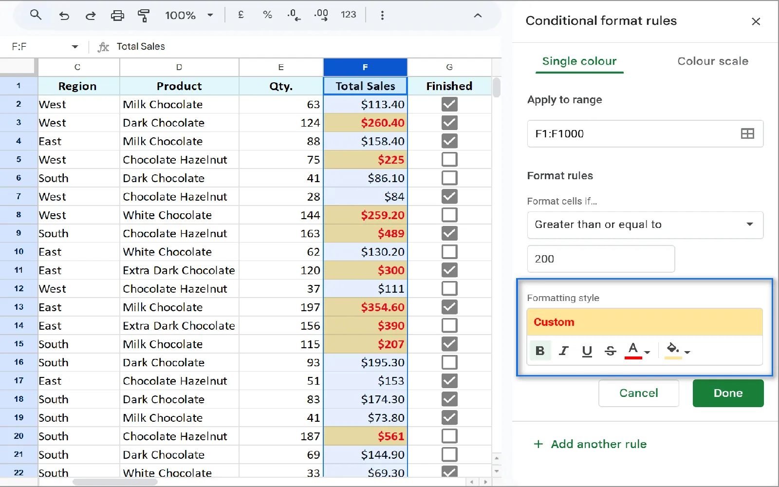
In the conditional formatting sidebar, you can define the rules based on your data. For instance, if you are working with ''referrerAdCreative'' metrics, you might want to highlight cells that exceed a certain threshold. Here’s how you can set up a simple rule:

1. Choose a format rule from the dropdown menu. For example, select Greater than.
2. Enter the value that serves as your threshold.
3. Choose a formatting style, such as changing the cell background color or text color.
4. Click Done to apply the rule.

This method allows you to quickly visualize which ''referrerAdCreative'' campaigns are performing well based on the metrics you’ve chosen.

Using Custom Formulas for Advanced Formatting

Conditional formatting can also utilize custom formulas for more advanced scenarios. This feature is particularly useful when you have complex datasets related to ''referrerAdCreative'' campaigns. To apply a custom formula, follow these steps:

1. In the conditional formatting sidebar, select Custom formula is from the dropdown menu.
2. Enter your formula. For example, if you want to highlight cells in column B where the value is greater than the corresponding value in column C, you would use a formula like =B1>C1.
3. Set the formatting style you prefer.
4. Click Done.

This flexibility enables you to create tailored visual cues that reflect the performance of each ''referrerAdCreative'' campaign, allowing for more insightful data analysis.

Examples of Conditional Formatting Applications

Let’s consider a few practical examples of how to use conditional formatting with ''referrerAdCreative'' data:

• Highlighting Top Performers: If you want to identify the top 10% of your ''referrerAdCreative'' campaigns based on click-through rates, you can create a rule that highlights the top percentage. Select your data range, choose Custom formula is, and enter =B1>=PERCENTILE(B:B, 0.9).
• Flagging Underperformers: Conversely, you can flag campaigns that fall below expectations by setting a rule that highlights cells where the value is less than a certain number, such as your average performance metric.
• Visualizing Trends: Use color scales to visualize changes over time. By applying a gradient color scale to your data, you can easily see which ''referrerAdCreative'' campaigns are improving or declining.

Combining Conditional Formatting with Charts

Another effective way to utilize conditional formatting is by combining it with charts. After applying conditional formatting to your data, you can create charts that reflect these visual cues. For example, if you have highlighted your top-performing ''referrerAdCreative'' campaigns, creating a chart based on this data will visually reinforce the insights gained from your formatting.

To create a chart, select the range of data you want to visualize and click on Insert in the menu, then choose Chart. Google Sheets will automatically suggest a chart type, but you can customize it further to suit your needs. The chart will now reflect any conditional formatting applied to your data, providing a comprehensive view of your campaign performance.

Best Practices for Using Conditional Formatting

While conditional formatting can greatly enhance data analysis, it’s essential to use it judiciously. Here are some best practices to keep in mind:

• Keep it Simple: Overusing conditional formatting can lead to confusion. Stick to a few key rules that provide the most value.
• Be Consistent: Use consistent color schemes and styles to avoid confusing interpretations of your data.
• Regularly Review Rules: As your data changes, regularly review and adjust your conditional formatting rules to ensure they remain relevant.

By following these best practices, you can maximize the benefits of conditional formatting in Google Sheets, especially when it comes to analyzing your ''referrerAdCreative'' campaigns.

Conclusion

Conditional formatting in Google Sheets is a versatile tool that can significantly enhance your data analysis capabilities. By learning to apply and customize conditional formatting rules, especially for ''referrerAdCreative'' data, you can gain valuable insights and make informed decisions. Whether you are a marketer, analyst, or business owner, mastering this feature will enable you to visualize your data effectively and drive better outcomes.